
Volumetric glassware
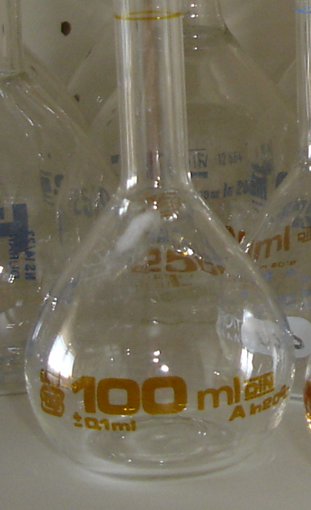
In analytical chemistry, it is important to work as accurately and precisely as possible. Therefore, almost all analytical, volumetric glassware shows the error that is made when using the glassware, such that you can calculate the size of the error in the experiment. An example is given in the picture below, which shows a close-up of a 100 mL volumetric flask. The error that you make when using this flask is ±0.1 mL.
Question: is this a random or systematic error?
In the remainder of this section, we will learn what this actually means and how it influences a final experimental result.
(Source: Wikipedia)
More on volumetric glassware
The error displayed on volumetric glassware is the random error resulting from the production process. In the case of the volumetric flask above, this would mean that a collection of identical flasks together has an error of ±0.1 mL (in other words: the standard deviation is 0.1 mL). However, individual flasks from the collection may have an error of +0.05 mL or -0.07 mL (Question: are these systematic or random errors?). For accurate results, you should constantly use different glassware such that errors cancel out. A second option is to calibrate the glassware: determine the volume by weighing. The error after calibration should be much smaller than the error shown on the glassware. Moreover, this error has now become random instead of systematic! Since this requires a lot of work each time you want to use volumetric glassware, we will from now on assume that errors shown on volumetric glassware are random errors. For example, each time when using the depicted volumetric flask properly, the volume will be 100 mL with an error of ±0.1 mL.
Significant figures
As a general rule, the last reported figure of a result is the first with uncertainty. Assume that we have measured the weight of an object: 80 kg. To indicate that we are not sure of the last digit,we can write 80 ± 1 kg. If we would have used a better scale to weigh the object, we might have found 80.00 ± 0.01 kg. Question: is the second result more precise or more accurate than the first?
We can also display the error in a relative way. For instance, 80 ± 1 kg is identical to 80 ± 1.25%. The order of magnitude of the result should be as clear as possible. Therefore, the preferred notation of for instance 0.0174 ± 0.0002 is (1.74 ± 0.02)·10-2.
Error propagation
When pipetting a volume with a certain pipette, the error in the final volume will be identical to the error shown on the pipette. But what happens to the error of the final volume when pipetting twice with the same pipette? Is it the same error as when using the pipette only once? And is there an error difference between using the same pipette twice or two times a different pipette? This becomes even more difficult when weighing a certain amount of salt and dissolving it in water to a certain volume. The error in weighing is shown on the scale and the error in volume on the volumetric flask, but what is the error in the density of this solution,  ?
?
Error propagation is able to answer all these questions. Basically, it it is a set of mathematical rules that explain how certain errors affect the final answer. Here, we will cover the most important and most used error propagation rules, including some practical examples.
Addition and subtraction
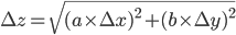
The rule for error propagation with addition and subtraction is as follows. If  , with
  and
and  being constants and
  ,
,  and
and  variables, the absolute error in is given by:
 ,
,  and
and  are the errors in , and , respectively.
Example 1: Suppose you pipette subsequently 10.00 ± 0.023 mL and 25.00 ± 0.050 mL in a beaker with uncalibrated pipettes. What is the error in the total volume of 35 mL?
Solution: In this example, = 10.00 mL, = 25.00 mL, = 35.00 mL, = 0.023 mL and = 0.050 mL. The total error can now be calculated via:
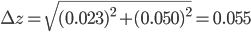
and are 1, because we use the two pipettes only once. The final answer is that you have pipetted 35.00 ± 0.055 mL.
Example 2: You pipette three times 10.00 ± 0.023 mL in a beaker with the same, uncalibrated pipette. What is the error in the total volume of 30 mL?
Solution: In this example, = 10.00 mL, = 0.023 mL and = 3. The total error can now be calculated:
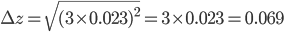
In the first example, two different pipettes were used. The errors made when pipetting with these pipettes are thus independent (they have nothing to do with each other). In the second example, the same pipette is used three times. Therefore, the errors in this example are dependent. The error is even exactly the same each time you pipette, because you are using the same pipette! That means that pipetting three times with the same pipette will lead to a bigger total error compared to pipetting three times with three different pipettes (indeed, errors cancel out to a certain extent in the latter case). This is exactly the reason that we are not allowed to add the errors in example 2 as we have done in example 1. Moreover, note that the repetition factor is also squared (Example 2).
Multiplication and division
The rule for error propagation with multiplication and division is: suppose that  or
or  , again with being a constant and , and variables. The relative error in is then given by:
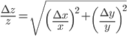
, and are the errors in , and , respectively.
Why do we use a relative error here and not an absolute error? The answer lies in the fact that, in the case of multiplication and division, and often represent different (physical) quantities, whereas with addition and subtraction and represent the same quantities (otherwise, we could not add them to begin with). You can for instance add two masses or subtract two volumes, but the addition of a mass and a volume is meaningless (e.g. what does '10 g + 3 mL' mean?). Division of mass and volume is not meaningless: it provides the density of a specific sample. The error in density cannot be calculated by simply adding the errors in mass and volume, because they are different quantities. That is why the total error is calculated with relative errors, which are unitless. The absolute error in can be calculated by multiplying the relative error, found with the rule above, with .
Example 3: You pipette 9.987 ± 0.004 mL of a salt solution in an Erlenmeyer flask and you determine the mass of the solution: 11.2481 ± 0.0001 g. What is the error in the density of the solution that can be calculated from these data?
Solution: In this case, = 11.2481 g, = 9.987 mL, = 0.0001 g and = 0.004 mL. The density can be calculated via  (compare ), thus
g·mL-1. The relative error equals:
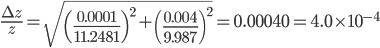
This means that the error in the final answer is 0.04% of the final answer itself. The absolute error can therefore be calculated via multiplication with :  . Using the right amount of significant figures, the final answer is that the density of the salt solution is equal to 1.1263 ± 0.0005 g·mL-1.
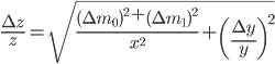
Example 4: Technically, the solution given above is not fully complete. The mass of a sample is always obtained by 'taring' the balance (i.e. setting the mass of the empty flask to 0). The obtained mass is therefore the difference between two masses:  . The error on such a balance, as also used during the practicals, is a random error. The total error when weighing can thus be obtained by using the error propagation rule for addition and subtraction. This total error should then be used to calculate the error in the density.
The weighing error is given by:

Final remarks
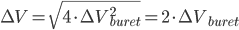
We have seen that a mass is always obtained as a difference between two masses: the error given on the balance can thus not be directly used in error propagation calculations (see Example 4). The same holds for a volume added via a burette: this is also the difference between an initial and a final volume and therefore the error propagation rule for addition and subtraction should be used. This becomes even worse when (correctly!) doing a titration: the blank (a difference between two volumes itself) should be subtracted from the result of an experiment (again a difference in two volumes). This results in a difference between two differences:  . Luckily, the total error in the volume can be calculated easily:
Continue with the questions on this subject.